An Analysis of Trump’s Tweets

Exploring tweets using the Racket programming language

Background

The following analysis uses several of my software tools under development, but is inspired by the work of David Robinson, and amounts to little more than a replication of his analysis shared on his blog Variance Explained. The long-term goal of this project is to make such analyses simple(r) by incorporating this workflow into an upcoming user-, and student-friendly analysis package called MassMine Analytics (or mmtool, as it’s temporarily known). Data for this analysis were collected using MassMine and the underlying tooling by my Racket data science package.

The Motivation

An astute twitter user noticed that when Trump said something positive, such as wish the Olympic team good luck, “he” tweeted from an iPhone (even though it is known that he uses a Samsung Galaxy). When his account tweets something negative, such as criticism for his opponents, it comes from an android device. This led to this analysis, recreated here with my own tooling, to determine if tweets from these two devices were categorically different–specifically, if his PR team was responsible for the iPhone-derived messages.

The Data Set

We will be working with tweets taken from Donald Trump’s Twitter account. The maximum we can collect from Twitter is his past 3200 tweets. With MassMine, getting this data is easy:

massmine --task=twitter-user --user=realDonaldTrump --count=3200 --out=trump_tweets.json

Preparing for the Analysis

To work with the resulting data (which is in JSON format), we load up a few tools in Racket scheme.

To begin, load the necessary dependencies

#lang racket

(require data-science)
(require plot)
(require math)
(require json)
(require pict)

Before we begin, we define several helper functions for parsing and working with the data set

;;; This function reads line-oriented JSON (as output by massmine),
;;; and packages it into an array. For very large data sets, loading
;;; everything into memory like this is heavy handed. For data this small,
;;; working in memory is simpler
(define (json-lines->json-array #:head [head #f])
  (let loop ([num 0]
             [json-array '()]
             [record (read-json (current-input-port))])
    (if (or (eof-object? record)
            (and head (>= num head)))
        (jsexpr->string json-array)
        (loop (add1 num) (cons record json-array)
              (read-json (current-input-port))))))

;;; Normalize case, remove URLs, remove punctuation, and remove spaces
;;; from each tweet. This function takes a list of words and returns a
;;; preprocessed subset of words/tokens as a list
(define (preprocess-text lst)
  (map (λ (x)
         (string-normalize-spaces
          (remove-punctuation
           (remove-urls
            (string-downcase x)))))
       lst))

Using Racket’s JSON package and the helper functions defined above, we can read in the tweet data (as raw JSON) and parse it as a list of hashes in Racket

;;; Read in the entire tweet database (3200 tweets from Trump's timeline)
(define tweets (string->jsexpr
                (with-input-from-file "trump_tweets.json" (λ () (json-lines->json-array)))))

Each tweet includes a lot of metadata. For this analysis we’ll keep only the text of each tweet, the timestamp from when it was posted online, along with its source–whether from an iPhone or Android device.

;;; Remove just the tweet text and source from each tweet
;;; hash. Finally, remove retweets.
;;; Remove just the tweet text, source, and timestamp from each tweet
;;; hash. Finally, remove retweets.
(define t
  (let ([tmp (map (λ (x) (list (hash-ref x 'text) (hash-ref x 'source)
                               (hash-ref x 'created_at))) tweets)])
    (filter (λ (x) (not (string-prefix? (first x) "RT"))) tmp)))

;;; Label each tweet as coming from iphone, android, or other.
(define tweet-by-type
  (map (λ (x) (list (first x)
                    (cond [(string-contains? (second x) "android") "android"]
                          [(string-contains? (second x) "iphone") "iphone"]
                          [else "other"])))
       t))

;;; Separate tweets by their source (created on iphone vs
;;; android... we aren't interested in tweets from other sources)
(define android (filter (λ (x) (string=? (second x) "android")) tweet-by-type))
(define iphone (filter (λ (x) (string=? (second x) "iphone")) tweet-by-type))

Results

Time of Tweets

If different people are using the android and iPhone device, we might expect a temporal signature related to when tweets are posted. We can visualize when tweets typically occur to confirm this suspicion:

;;; Helper function for converting raw JSON timestamps to something we
;;; can use
(define (convert-timestamp str)
  (string->date str "~a ~b ~d ~H:~M:~S ~z ~Y"))

;;; Timestamps by device
(define timestamp-by-type
  (map (λ (x) (list (third x)
                    (cond [(string-contains? (second x) "android") "android"]
                          [(string-contains? (second x) "iphone") "iphone"]
                          [else "other"])))
       t))

;;; Timestamp binning. Simple counts of data records by unit time.
(define (bin-timestamps timestamps)
  (let ([time-format "~H"])
    ;; Return
    (sorted-counts
     (map (λ (x) (date->string (convert-timestamp x) time-format)) timestamps)))) 

;;; Android binned times
(define a-time
  (bin-timestamps ($ (subset timestamp-by-type 1 (λ (x) (string=? x "android"))) 0)))
;;; iPhone binned times
(define i-time
  (bin-timestamps ($ (subset timestamp-by-type 1 (λ (x) (string=? x "iphone"))) 0)))

;;; Convert bin names to numbers
(define a-time (map (λ (x) (list (string->number (first x)) (second x))) a-time))
(define i-time (map (λ (x) (list (string->number (first x)) (second x))) i-time))

;;; Fill in missing data. This helper makes sure we have a bin for
;;; every hour, even if zero tweets were observed. `bins` should
;;; contain a list of all required bins. Missing bins will be filled
;;; with a zero
(define (fill-missing-bins lst bins)
  (define (get-count lst val)
    (let ([count (filter (λ (x) (equal? (first x) val)) lst)])
      (if (null? count) (list val 0) (first count))))
  (map (λ (bin) (get-count lst bin))
       bins))

;;; Convert UTC time to EST
(define (time-EST lst)
  (map list
       ($ lst 0)
       (append (drop ($ lst 1) 4) (take ($ lst 1) 4))))

;;; Convert bin counts to percentages
(define (count->percent lst)
  (let ([n (sum ($ lst 1))])
    (map list
         ($ lst 0)
         (map (λ (x) (* 100 (/ x n))) ($ lst 1)))))

;;; What time of day do the different devices tend to tweet?
(let ([a-data (count->percent (time-EST (fill-missing-bins a-time (range 24))))]
      [i-data (count->percent (time-EST (fill-missing-bins i-time (range 24))))])
  (parameterize ([plot-legend-anchor 'top-right]
                 [plot-width 600])
      (plot (list
             (tick-grid)
             (lines a-data
                    #:color "OrangeRed"
                    #:width 2
                    #:label "Android")
             (lines i-data
                    #:color "LightSeaGreen"
                    #:width 2
                    #:label "iPhone"))
            #:x-label "Hour of day (EST)"
            #:y-label "% of tweets")))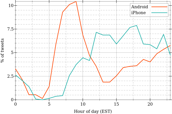

Trump’s Quotations

A quick look at Trump’s Twitter timeline reveals that many tweets quote someone else. We can plot what proportion of tweets from each device consist of quotations versus original content:

;;; Let's count how many tweets were quotes of someone else from both
;;; sources.
(define android-quotes
  (let ([quotes (map (λ (x) (if (string-prefix? x "\"") "Quoted" "Not Quoted"))
                     ($ android 0))])
    (let-values ([(label n) (count-samples quotes)])
      (map list label n))))
(define iphone-quotes
  (let ([quotes (map (λ (x) (if (string-prefix? x "\"") "Quoted" "Not Quoted"))
                     ($ iphone 0))])
    (let-values ([(label n) (count-samples quotes)])
      (map list label n))))

;;; Restructure the data for our histogram below
(define quoted
  (list `("Android" ,(second (first android-quotes)))
        `("iPhone" ,(second (second iphone-quotes)))))
(define not-quoted
  (list `("Android" ,(second (second android-quotes)))
        `("iPhone" ,(second (first iphone-quotes)))))


;;; Plot number of quoted vs unquoted tweets per device
(plot (list (discrete-histogram not-quoted
                                #:label "Not Quoted"
                                #:skip 2.5
                                #:x-min 0
                                #:color "OrangeRed"
                                #:line-color "OrangeRed")
            (discrete-histogram quoted
                                #:label "Quoted"
                                #:skip 2.5
                                #:x-min 1
                                #:color "LightSeaGreen"
                                #:line-color "LightSeaGreen"))
      #:y-max 1500
      #:x-label ""
      #:y-label "Number of tweets")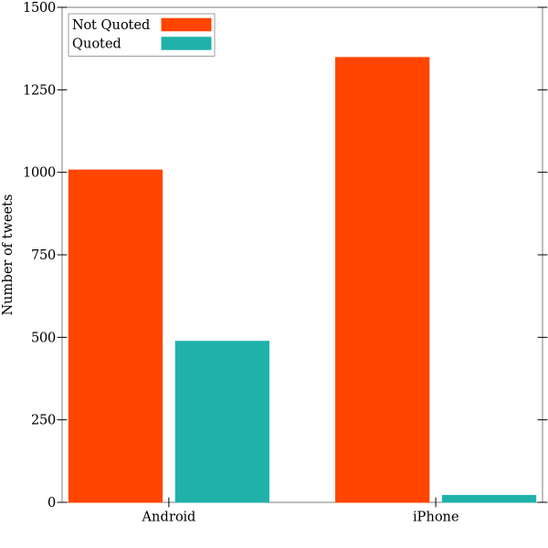

This figure demonstrates clearly that the iPhone user generates almost entirely novel content. Many tweets from this device function as press releases, announcements for upcoming events, etc.

Linked Content (Images)

Moving forward, we want to focus on tweets containing novel content (the red-orange bars in the figure above). We remove any tweet beginning with quotation marks.

;;; From here foward, we remove quoted tweets to focus exclusively on
;;; content unique to the Trump twitter feed
(define android
  (filter (λ (x) (not (string-prefix? (first x) "\""))) android))
(define iphone
  (filter (λ (x) (not (string-prefix? (first x) "\""))) iphone))

Trump’s Twitter account often shares images and links related to campaign events. Is this content shared equally across devices?

;;; Next we count how may tweets from each device links to an image
(define android-pics
  (let ([pics (map (λ (x)
                     (if (string-contains? x "t.co")
                         "Picture/Link"
                         "No picture/link"))
                   ($ android 0))])
    (let-values ([(label n) (count-samples pics)])
      (map list label n))))
(define iphone-pics
  (let ([pics (map (λ (x)
                     (if (string-contains? x "t.co")
                         "Picture/Link"
                         "No picture/link"))
                   ($ iphone 0))])
    (let-values ([(label n) (count-samples pics)])
      (map list label n))))

;;; Restructure the data for our histogram below
(define pics
  (list `("Android" ,(second (second android-pics)))
        `("iPhone" ,(second (second iphone-pics)))))
(define no-pics
  (list `("Android" ,(second (first android-pics)))
        `("iPhone" ,(second (first iphone-pics)))))

;;; Finally, we can plot the ratio of tweets with pics to no pics
(parameterize ([plot-legend-anchor 'top-right])
  (plot (list (discrete-histogram no-pics
                                  #:label "No picture/link"
                                  #:skip 2.5
                                  #:x-min 0
                                  #:color "OrangeRed"
                                  #:line-color "OrangeRed")
              (discrete-histogram pics
                                  #:label "Picture/link"
                                  #:skip 2.5
                                  #:x-min 1
                                  #:color "LightSeaGreen"
                                  #:line-color "LightSeaGreen"))
        #:y-max 1100
        #:x-label ""
        #:y-label "Number of tweets"))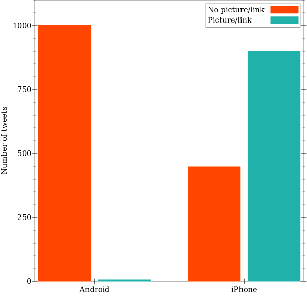

Once again, we see a distinct pattern. The iPhone device shares a rich amount of media content, typically similar to the following:

PHOTO REMOVED FROM TWITTER

Most Common Words Across Devices

For the remaining analysis, we’ll perform text-level analyses. To begin, we clean up using typical text-processing strategies: remove case, URLs, punctuation, stop-words, and extra spaces. Then we split tweets into words and combine across tweets for each device, as well as for both devices combined.

Finally, we plot the 20 most frequent words used across both devices.

;;; Normalize case, remove URLs, remove punctuation, and remove spaces
;;; from each tweet. 
(define (preprocess-text str)
  (string-normalize-spaces
   (remove-punctuation
    (remove-urls
     (string-downcase str)) #:websafe? #t)))

(define a (map (λ (x)
                 (remove-stopwords x))
               (map (λ (y)
                      (string-split (preprocess-text y)))
                    ($ android 0))))

(define i (map (λ (x)
                 (remove-stopwords x))
               (map (λ (y)
                      (string-split (preprocess-text y)))
                    ($ iphone 0))))

;;; Remove empty strings and flatten tweets into a single list of
;;; words 
(define a (filter (λ (x) (not (equal? x ""))) (flatten a)))
(define i (filter (λ (x) (not (equal? x ""))) (flatten i)))
;;; All words from both sources of tweets
(define b (append a i))
;;; Only words that are used by both devices
(define c (set-intersect a i))

;; ;;; Word list from android and iphone tweets
(define awords (sort (sorted-counts a)
                     (λ (x y) (> (second x) (second y))))) 
(define iwords (sort (sorted-counts i)
                     (λ (x y) (> (second x) (second y)))))
(define bwords (sort (sorted-counts b)
                     (λ (x y) (> (second x) (second y)))))

;;; Plot the top 20 words from both devices combined
(parameterize ([plot-width 600]
               [plot-height 600])
    (plot (list
        (tick-grid)
        (discrete-histogram (reverse (take bwords 20))
                            #:invert? #t
                            #:color "DimGray"
                            #:line-color "DimGray"
                            #:y-max 450))
       #:x-label "Occurrences"
       #:y-label "word"))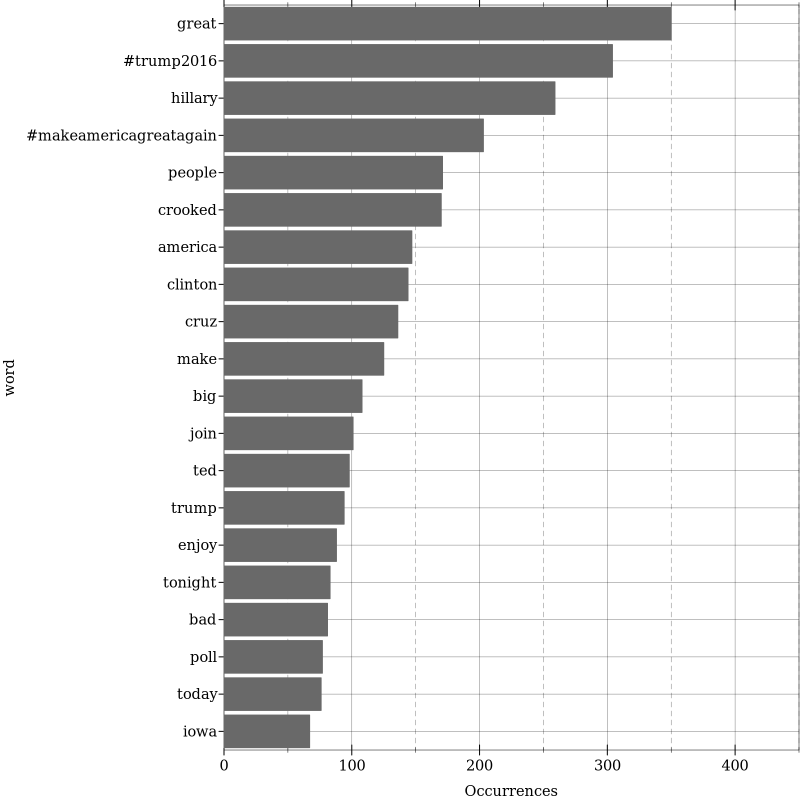

These terms should be familiar if you’ve been following the Trump spin machine. Even more interesting is a comparison between the words from the android vs iPhone devices. We use log-odds (to overcome the asymmetric nature of data from ratios).

;;; Now we calculate the log odds ratio of words showing up in tweets
;;; across both devices
(define (get-word-freq w lst)
  (let ([word-freq (filter (λ (x) (equal? (first x) w)) lst)])
    (if (null? word-freq) 0 (second (first word-freq)))))

;;; Next, calculate the log odds for the top-20 words from the
;;; android, and then the log odds for the top-20 words from the
;;; iphone. 
(define log-odds
  (map (λ (x)
         `(,x
           ,(log-base (/
                       (/ (add1 (get-word-freq x awords)) (add1 (length a)))
                       (/ (add1 (get-word-freq x iwords)) (add1 (length i))))
                      #:base 2)))
       c))

;;; Plot the results
(let ([android-words (take (sort log-odds (λ (x y) (> (second x) (second y)))) 20)]
      [iphone-words (take (sort log-odds (λ (x y) (< (second x) (second y)))) 20)])
  (parameterize ([plot-width 600]
                 [plot-height 600])
      (plot (list
             (discrete-histogram iphone-words
                                 #:invert? #t
                                 #:y-min -7.5
                                 #:y-max 5
                                 #:color "LightSeaGreen"
                                 #:line-color "LightSeaGreen")
             (discrete-histogram (reverse android-words)
                                 #:invert? #t
                                 #:x-min 20
                                 #:y-min -7.5
                                 #:y-max 5
                                 #:color "OrangeRed"
                                 #:line-color "OrangeRed"))
            #:x-label "Android / iPhone log ratio"
            #:y-label "word")))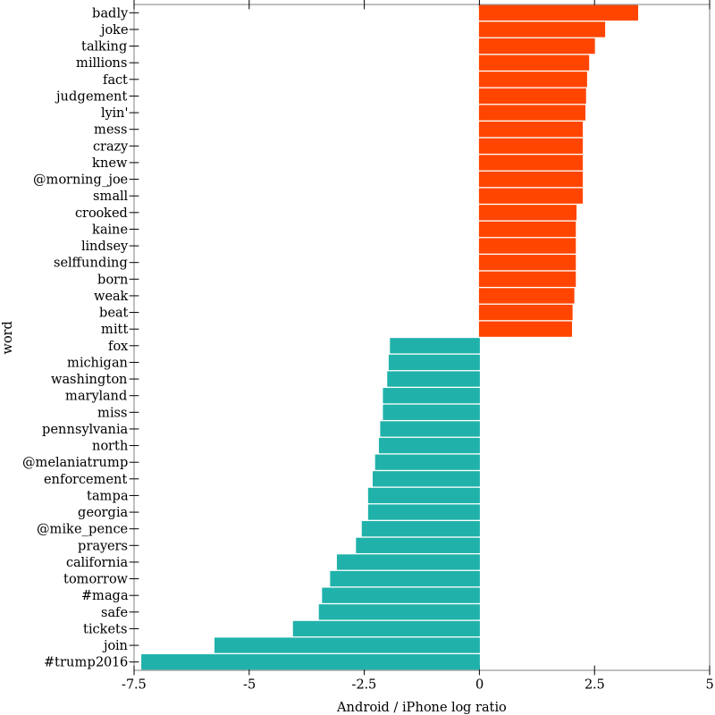

In the above figure, positive log-odds reflect words more commonly found in android tweets, with negative log ratios for words more common in iPhone-derived tweets. A quick visual scan reveals a clear distinction between the two groups of tweets. The iPhone features campaign slogans and hashtags, dates, and event information. The android account does not, by comparison, but does feature many more emotionally-charged words.

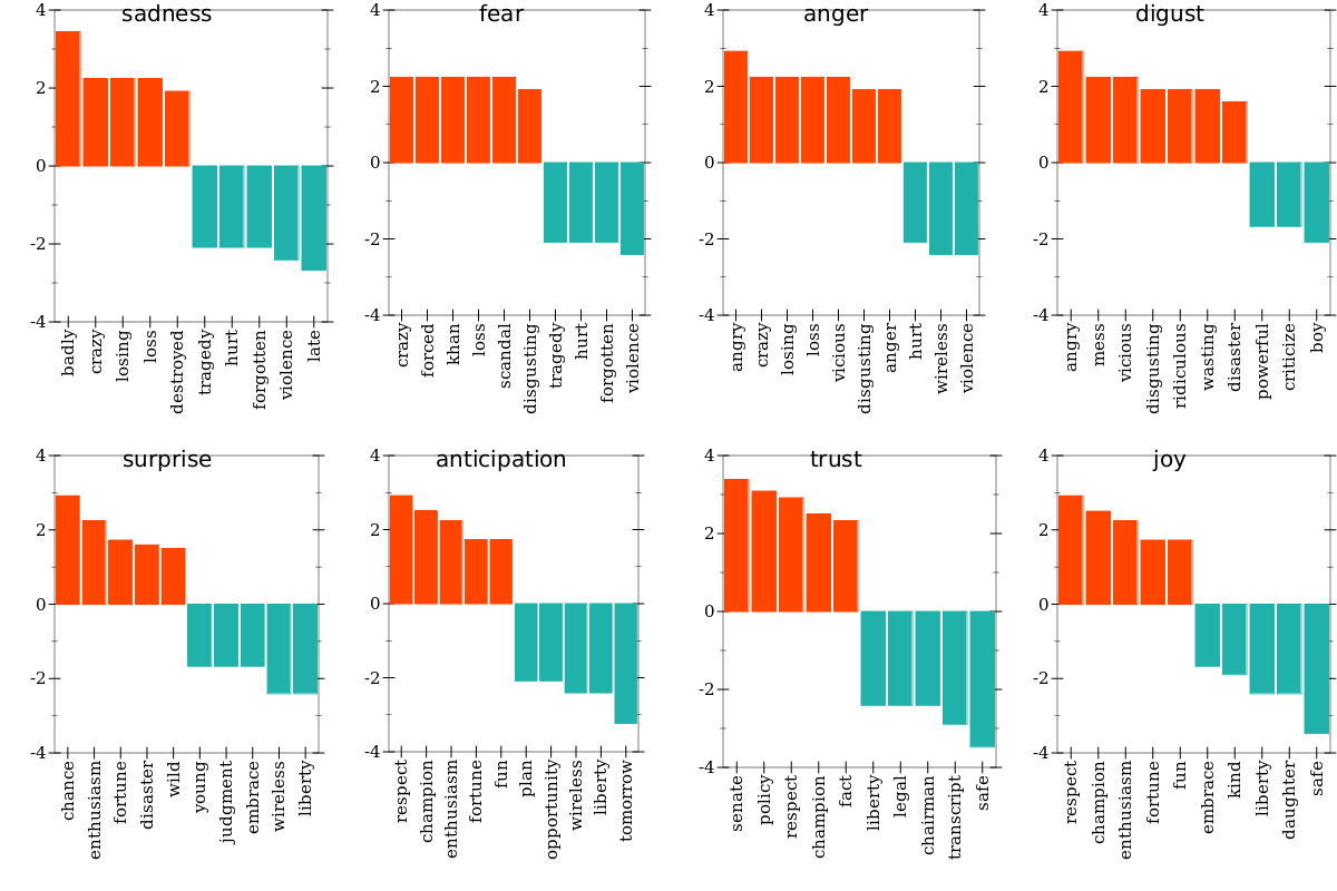
Sentiment Analysis

In the figure above, the top words suggest a difference in sentiment, or emotional valence between the two devices. We can assess this further with sentiment analysis by assigning an affective label to each word in the tweets. Words are assigned one of the following labels (or none at all):

• sadness
• fear
• anger
• surprise
• anticipation
• trust
• joy

By tabulating the frequency of sentiment scores, we can inspect the top 10 most influential words from each emotional label, and determine whether they occur most frequently in android vs iPhone tweets.

;;; Sentiment from words coming from either device
(define bsentiment (filter (λ (x) (second x)) (list->sentiment bwords #:lexicon 'nrc)))

;;; We calculate the log odds for each affective label from the
;;; sentiment analysis
(define (find-sentiment-log-odds str)
  (map (λ (x)
         `(,x
           ,(log-base (/
                       (/ (add1 (get-word-freq x awords)) (add1 (length a)))
                       (/ (add1 (get-word-freq x iwords)) (add1 (length i))))
                      #:base 2)))
       ($ (subset bsentiment 1 (λ (x) (string=? x str))) 0)))

;;; Apply the above helper to each affective label
(define sadness-lo (find-sentiment-log-odds "sadness"))
(define fear-lo (find-sentiment-log-odds "fear"))
(define anger-lo (find-sentiment-log-odds "anger"))
(define disgust-lo (find-sentiment-log-odds "disgust"))
(define surprise-lo (find-sentiment-log-odds "surprise"))
(define anticipation-lo (find-sentiment-log-odds "anticipation"))
(define trust-lo (find-sentiment-log-odds "trust"))
(define joy-lo (find-sentiment-log-odds "joy"))

;;; Helper plotting function
(define (plot-sentiment lst)
  (let* ([n (min 10 (length lst))]
         [top-words (take (sort lst (λ (x y) (> (abs (second x)) (abs (second y))))) n)]
         [android-words (filter (λ (x) (positive? (second x))) top-words)]
         [iphone-words (filter (λ (x) (negative? (second x))) top-words)])
    (parameterize ([plot-width 300]
                   [plot-height 400]
                   [plot-x-tick-label-anchor 'right]
                   [plot-x-tick-label-angle 90])
      (plot-pict (list
                  (discrete-histogram android-words
                                      #:y-min -4
                                      #:y-max 4
                                      #:color "OrangeRed"
                                      #:line-color "OrangeRed")
                  (discrete-histogram (reverse iphone-words)
                                      #:x-min (length android-words)
                                      #:y-min -4
                                      #:y-max 4
                                      #:color "LightSeaGreen"
                                      #:line-color "LightSeaGreen"))
                 #:x-label ""
                 #:y-label ""))))

;;; Plot everything together
(vl-append
 (hc-append (ct-superimpose (plot-sentiment sadness-lo) (text "sadness" null 20))
            (ct-superimpose (plot-sentiment fear-lo) (text "fear" null 20))
            (ct-superimpose (plot-sentiment anger-lo) (text "anger" null 20))
            (ct-superimpose (plot-sentiment disgust-lo) (text "digust" null 20)))
 (hc-append (ct-superimpose (plot-sentiment surprise-lo) (text "surprise" null 20))
            (ct-superimpose (plot-sentiment anticipation-lo) (text "anticipation" null 20))
            (ct-superimpose (plot-sentiment trust-lo) (text "trust" null 20))
            (ct-superimpose (plot-sentiment joy-lo) (text "joy" null 20))))